
In this section, the method of least squares will be used to find data reduction algorithms with maximal signal to noise ratio. Least squares methods have been extensively used in X-ray astronomy. Justification for the use of these methods, and their limitations when applied to Poisson distributed data have been discussed in the literature (refs).
The coded aperture camera is a linear system whose response may be described by the matrix equation:
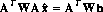
The raw measurements are a histogram of events with expectation values given by the column vector $h$. The column vector $x$ represents the (unknown) source fluxes and background flux, while the matrix $A$ represents the behavior of the camera. Each column of $A$ represents the response of the camera to a unit flux from the corresponding source. Given an actual measured histogram, $h$, we may estimate the unknowns by solving the equation:

The vector $x hat$ is an estimate of $x$. If $sigma sup 2$ represents the variance of each element of $h$, then the matrix $sigma sup 2 ( bold A sup T bold A ) sup -1$ (the "covariance" or "error" matrix) represents the covariances of the elements of $x hat$. In particular, the diagonal elements of the error matrix are the variances of the elements of $x hat$ (Refs.). In practice, since we must normally estimate the variance of actual measured data, the error matrix must be considered an estimate of the true covariances.
The error matrix technique is especially useful when comparing the performance of different camera designs, since it allows the designer to avoid extensive Monte-Carlo testing. In this case, variances may be accurately calculated rather than estimated.
If different observations have different variances, the a weighted least squares method is appropriate:
$W$ is a diagonal matrix of "weights"; each diagonal element of $W$ should be the inverse of the variance of the corresponding observation. Since for Poisson statistics, the variance and expectation value are the same:

Unfortunately, this equation cannot be applied directly to actual data since $h$ isn't something that can be measured.
Thus, a way to estimate the appropriate weights is needed. Possible methods include:
The success of the above methods depends on the observed fact that in most practical cases, the results are only weakly dependent on the weights. Methods (1) and (2) misbehave for small numbers of counts, when $W$ becomes extremely dependent on the data. Note that if the number of counts is large, methods (1) and (2) are nearly linear in the data, and method (3) is exactly linear.
Criteria for determining confidence intervals for estimates based on method (2) have been described in the literature. These criteria are applicable in both nonlinear and linear cases. In the case of a linear or nearly linear method, it is often more convenient to use the error matrix to estimate the signal to noise ratio. If the weight matrix $W$ accurately represents the inverses of the variances of $h$, then the matrix $( A sup T W A ) sup -1$ is the error matrix for the weighted method.
The solution to the weighted lest squares method may be written:

where:
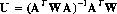
This is closely related to Fenimore's "URA-tagging" method for coded aperture photometry. Individual elements of $x$ may be computed by computing the dot product of the corresponding row of $U$ with the measurements $h$. In Fenimore's terminology, the rows of $U$ are "tag arrays". Thus, an individual source intensity may be efficiently computed if its tag array is known beforehand. This is especially true if $h$ is sparse, which in this case means that it contains many fewer photons than elements. Fenimore suggests forming the dot product photon by photon in such cases: this is essentially the well known technique for multiplying a "randomly packed" sparse matrix by another matrix.
The least squares method described above provides a straightforward way to calculate tag arrays which yield optimal signal to noise. The method also demonstates that "URA tagging" is not restricted to URA based cameras: the special properties of the URA were not invoked at any point in the derivation.
An important special case is the case where there is just one source and no weighting is needed. In this case, the matrix $A$ is reduced to a vector, $a$, and the vector $x$ is reduced to a scalar, $x$. The least squares estimate of $x$ is just the correlation of $a$ with the data, $h$, normalized by dividing by the correlation of $a$ with itself:

This result demonstrates the "matched filter" principle: the optimum way to detect a signal in noisy data is to correlate the data with the expected signal. This principle is applicable whenever the noise is of constant amplitude ($sigma sup 2 ( h sub i ) ~=~ sigma sup 2 ( h sub j )$), and the noise in separate measurements is uncorrelated.
The error "matrix" is just the scalar $ { sigma sup 2 } over { bold a cdot bold a }$. Since this is the variance of $x hat$, its square root represents the noise in the measurement. The signal to noise ratio is thus:

The correlation of $a$ with itself, $a cdot a$, represents the signal power which results from a source of unit flux. Keeping track of the signal power will prove to be an effective way to understand the sensitivity of coded aperture cameras.